(GRE - sequence) A
gradient echo is generated by using a pair of bipolar
gradient pulses. In the
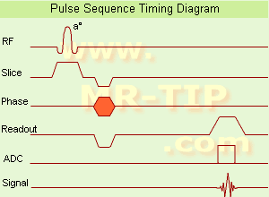
pulse sequence timing diagram, the basic
gradient echo sequence is illustrated. There is no
refocusing 180° pulse and the data are sampled during a
gradient echo, which is achieved by
dephasing the spins with a negatively pulsed
gradient before they are rephased by an opposite
gradient with opposite polarity to generate the
echo.
See also the
Pulse Sequence Timing Diagram. There you will find a description of the components.
The
excitation pulse is termed the alpha pulse α. It tilts the
magnetization by a
flip angle α, which is typically between 0° and 90°. With a small
flip angle there is a reduction in the value of
transverse magnetization that will affect subsequent RF pulses.
The
flip angle can also be slowly increased during data acquisition (variable flip angle: tilt optimized nonsaturation
excitation).
The data are not acquired in a steady state, where z-magnetization recovery and destruction by ad-pulses are balanced.
However, the z-magnetization is used up by tilting a little more of the remaining z-magnetization into the xy-plane for each acquired imaging line.
Gradient echo imaging is typically accomplished by examining the
FID, whereas the read
gradient is turned on for localization of the signal in the readout direction.
T2* is the characteristic
decay time constant associated with the
FID. The
contrast and signal generated by a
gradient echo depend on the size of the
longitudinal magnetization and the
flip angle.
When α = 90° the sequence is identical to the so-called
partial saturation or
saturation recovery pulse sequence.
In standard GRE imaging, this basic
pulse sequence is repeated as many times as image lines have to be acquired.
Additional
gradients or
radio frequency pulses are introduced with the aim to spoil to refocus the xy-magnetization at the moment when the
spin system is subject to the next α pulse.
As a result of the short
repetition time, the z-magnetization cannot fully recover and after a few initial α pulses there is an
equilibrium established between z-magnetization recovery and z-magnetization reduction due to the α pulses.
Gradient echoes have a lower SAR, are more sensitive to field inhomogeneities and have a reduced crosstalk, so that a small or no
slice gap can be used.
In or
out of phase imaging depending on the
selected TE (and
field strength of the
magnet) is possible.
As the
flip angle is decreased, T1 weighting can be maintained by reducing the TR.
T2* weighting can be minimized by keeping the TE as short as possible, but pure T2 weighting is not possible.
By using a reduced
flip angle, some of the
magnetization value remains longitudinal (less time needed to achieve full recovery) and for a certain T1 and TR, there exist one
flip angle that will give the most signal, known as the "Ernst angle".
Contrast values:
PD weighted: Small
flip angle (no T1), long TR (no T1) and short TE (no
T2*)
T1 weighted: Large
flip angle (70°), short TR (less than 50ms) and short TE
T2* weighted: Small
flip angle, some longer TR (100 ms) and long TE (20 ms)
Classification of GRE sequences can be made into four categories:
See also
Gradient Recalled Echo Sequence,
Spoiled Gradient Echo Sequence,
Refocused Gradient Echo Sequence,
Ultrafast Gradient Echo Sequence.


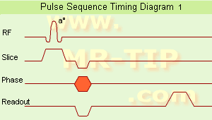 The schematic figures of a
 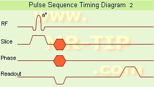 The
The